Week 4: Data manipulation and statistical analysis in R
University of New South Wales
School of Risk and Actuarial Studies
Term 2 2021
Learning outcomes
By the end of this topic, you should be able to
extract elements from different R data structures in an efficient way
manipulate different types of R data structures with appropriate R functions
summarise and organise data in a variety of ways
compute statistics from data
Data frame example
Y <- data.frame(GENDER=c("F","M","M","F"),
Height=c(165,182,178,160),
Weight=c(50,65,67,55),
Income=c(80,90,60,50))
row.names(Y)<-c('Aiyana','James','John','Abbey')
Y
## GENDER Height Weight Income
## Aiyana F 165 50 80
## James M 182 65 90
## John M 178 67 60
## Abbey F 160 55 50
Y[3,2]
## [1] 178
Y['John','Height']
## [1] 178
Y$Weight
## [1] 50 65 67 55
Y['John',]
## GENDER Height Weight Income
## John M 178 67 60
Y[,'Height']
## [1] 165 182 178 160
Data frame - Exercise
- What is the average income of the males?
- What is the weight of Abbey?
Data frame - Solution
Y <- data.frame(GENDER=c("F","M","M","F"),
Height=c(165,182,178,160),
Weight=c(50,65,67,55),
Income=c(80,90,60,50))
row.names(Y)<-c('Aiyana','James','John','Abbey')

mean(Y$Income[Y$GENDER == "M"])
## [1] 75
Y['Abbey','Weight']
## [1] 55
The attach() function
- The function
attach(some.data.frame) creates a workspace where each variable of the data frame can be accessed directly (without using the dollar sign $). Therefore it can reduce the length of codes. However, this space does not ‘communicate’ with the working directory. Therefore, if you make a change in the data frame, it will not be effective in this additional workspace.
- We recommend to be very careful with the
attach() function (especially for large projects).
attach(Y)
GENDER
## [1] "F" "M" "M" "F"
# We update GENDER in our data frame X
Y$GENDER <- c("F", "F", "F", "F")
Y$GENDER
## [1] "F" "F" "F" "F"
# However, the version of X we 'attached' has NOT been updated
GENDER
## [1] "F" "M" "M" "F"
Statistical Analysis - Importing data - Pages 339-343
Here we use the sample_data.csv data to illustrate a few handy statistical functions. This data is already in Ed (in this week’s “Lab Exercise Space”). You can download it if you want to use it on your computer.
- import the data to R (if doing this on your computer, first save the data in the folder you set as the working directory)
- use the
attach() function to gain direct access to the variables
sample_data <- read.csv("sample_data.csv", header=TRUE)
attach(sample_data)
head(sample_data)
##   X gender situation tea coffee height weight age      meat      fish raw_fruit
## 1 1 Female    single   0      0    151     58  58 4-6/week. 2-3/week.  <1/week.
## 2 2 Female    single   1      1    162     60  60    1/day.   1/week.    1/day.
## 3 3 Female    single   0      4    162     75  75 2-3/week.  <1/week.    1/day.
## 4 4 Female    single   0      0    154     45  45     never 4-6/week. 4-6/week.
## 5 5 Female    single   2      1    154     50  50    1/day. 2-3/week.    1/day.
## 6 6 Female    single   2      0    159     66  66 4-6/week.   1/week.    1/day.
##   cooked_fruit_veg    chocol       fat
## 1        4-6/week.    1/day.     Isio4
## 2           1/day.  <1/week. sunflower
## 3          1/week.    1/day. sunflower
## 4            never 2-3/week. margarine
## 5           1/day. 2-3/week. margarine
## 6           1/day.  <1/week.    peanut
Statistical Analysis - Variables - Pages 339-343
\(13\) variables (columns) of \(226\) individuals (rows)
qualitative: gender, situation and fat
ordinal: meat, fish, raw_fruit, cooked_fruit_veg and chocol
discrete quantitative: tea, coffee
continuous quantitative: height, weight and age
Notes
The sample_data.csv is created based from the nutrition_elderly.csv spreadsheet downloaded from http://www.biostatisticien.eu/springeR/nutrition_elderly.xls. See Page 339.
Variables of nutrition_elderly.csv have been structured following the steps from Pages 340-343 and a new data frame was created and saved as sample_data.csv.
Numerical statistics - Pages 347-352
Some useful statistics for a preliminary analysis (of variable weight in this example):
mean(weight)
## [1] 66.4823
median(weight)
## [1] 66
sd(weight)
## [1] 12.03337
max(weight)-min(weight)
## [1] 58
IQR(weight)
## [1] 17.75
mean(abs(weight-mean(weight)))
## [1] 9.919884
quantile(weight, probs=c(0.1,0.9))
##  10%  90%
## 51.5 82.0
Note: Remember, variable weight can be accessed directly only because we use the command attach(sample_data) previously!
Exercise
Use the built-in dataset women. Provide the following summary statistics for the height of women.
mean
median
standard deviation
range
25% and 75% quantiles
Solution
mean(women$height)
## [1] 65
median(women$height)
## [1] 65
sd(women$height)
## [1] 4.472136
max(women$height)-min(women$height)
## [1] 14
quantile(women$height, probs=c(0.25,0.75))
##  25%  75%
## 61.5 68.5
Frequency table - discrete variables - Pages 343-344
For qualitative variable fat:
(tc <- table(fat))
## fat
##    butter      duck     Isio4 margarine     olive    peanut repesseed sunflower
##        15         4        23        27        40        48         1        68
(tf <- tc/length(fat))
## fat
##      butter        duck       Isio4   margarine       olive      peanut
## 0.066371681 0.017699115 0.101769912 0.119469027 0.176991150 0.212389381
##   repesseed   sunflower
## 0.004424779 0.300884956
Frequency table - joint observations - Pages 344-345
For the paired observations of gender and situation:
(mytable <- table(gender,situation))
##         situation
## gender   couple family single
##   Female     56      7     78
##   Male       63      2     20
(table.complete <- addmargins(mytable, FUN=sum, quiet=TRUE))
##         situation
## gender   couple family single sum
##   Female     56      7     78 141
##   Male       63      2     20  85
##   sum       119      9     98 226
Correlation: an association measure - Pages 354-355
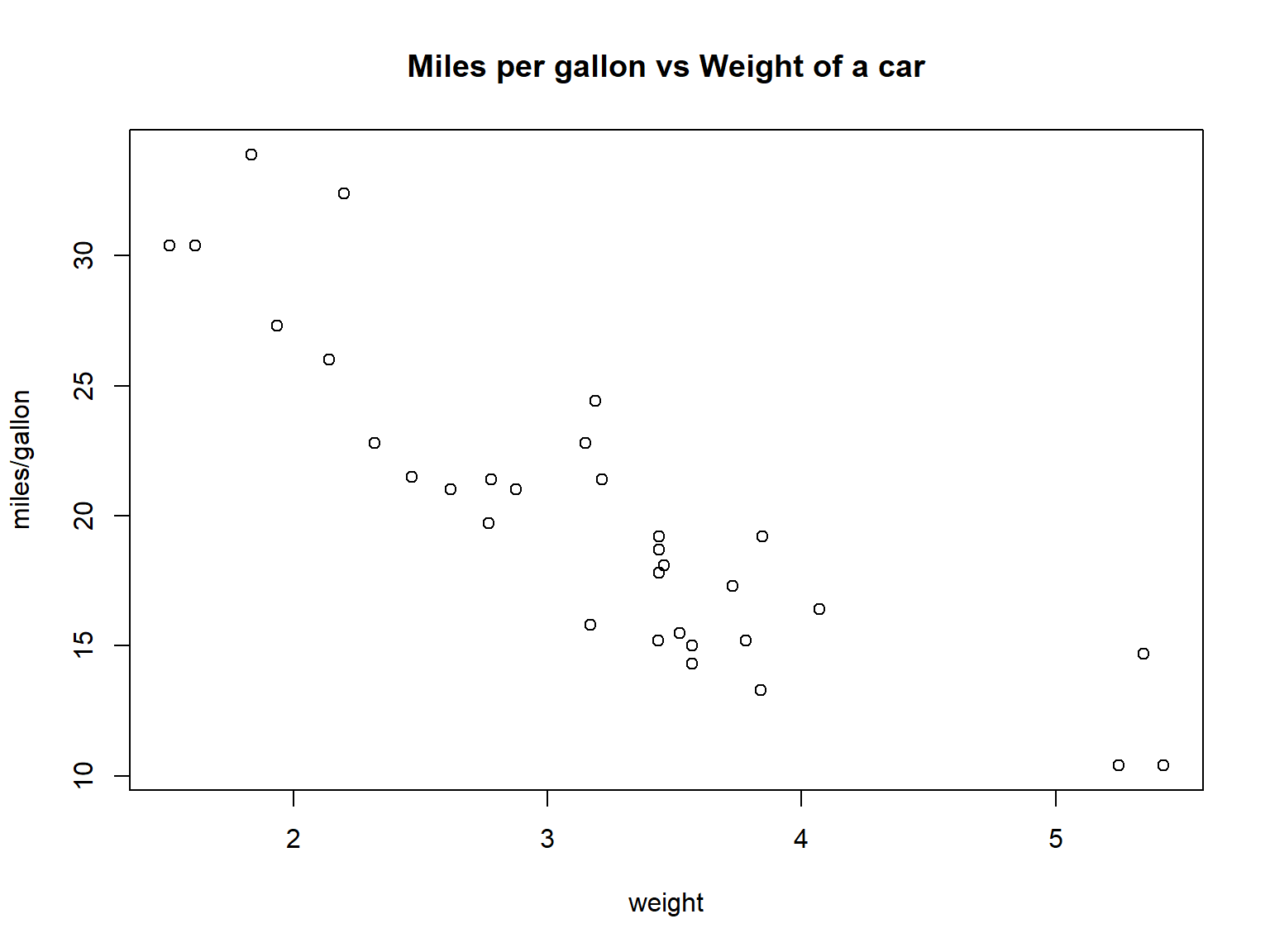
The cor() function computes the (sample) correlation between two variables, which is a measure of linear association. As an example, we compute the correlation between two variables from the in-built dataset mtcars:
wt: weight of the car (in 1000’s of pounds)mgp: miles per gallon
cor(mtcars$wt, mtcars$mpg)
## [1] -0.8676594
The correlation always ranges from \(-1\) to \(1\). Here a correlation of \(-0.868\) indicates a strong negative association between wt and mgp: the heavier the car, the less distance it can go with one gallon of fuel (which makes sense!).
Note: We will see more about correlation in Module 4: Risk & Insurance (Theory component of the course).
Exercise
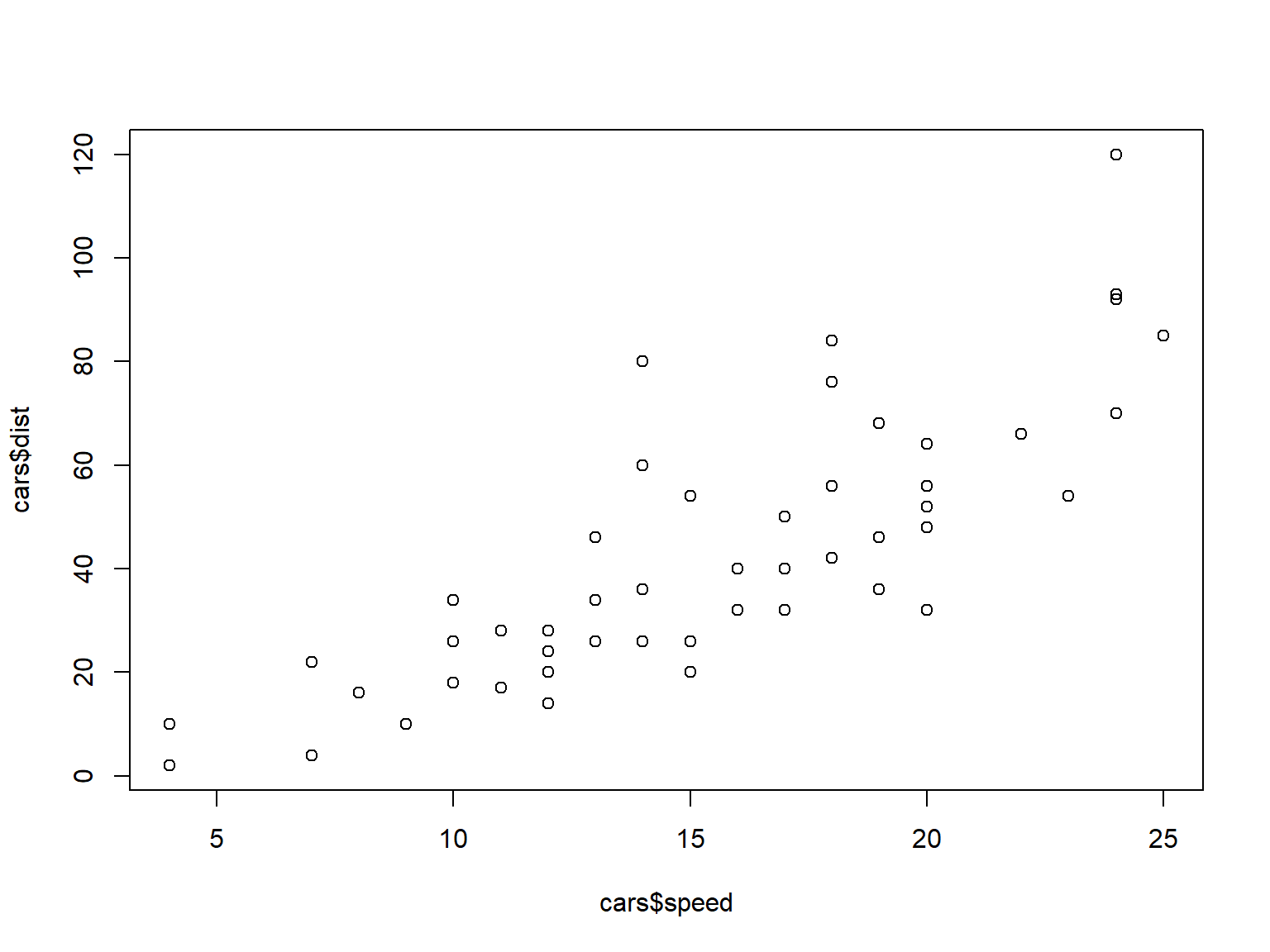
Use the in-built R dataset cars. Calculate the correlation between the speed and dist (for stopping distance) from the 50 observations.
What can you learn? Is there any further investigation you want to do?
Solution
cor(cars$speed, cars$dist)
## [1] 0.8068949
Comments:
The correlation is \(0.807\), which indicates a high level of positive linear association between the two variables, i.e. if one variable is “high”, the other variable also tends to be “high”.
We can create the scatter plot of one variable versus the other and examine the relationship ‘visually’. More on plots next Week!
Here it turns out that an even better description of the relationship between these two variables is a linear relationship between the log-scaled values… also more on that later!
plot(cars$speed, cars$dist)
plot(log(cars$speed), log(cars$dist))
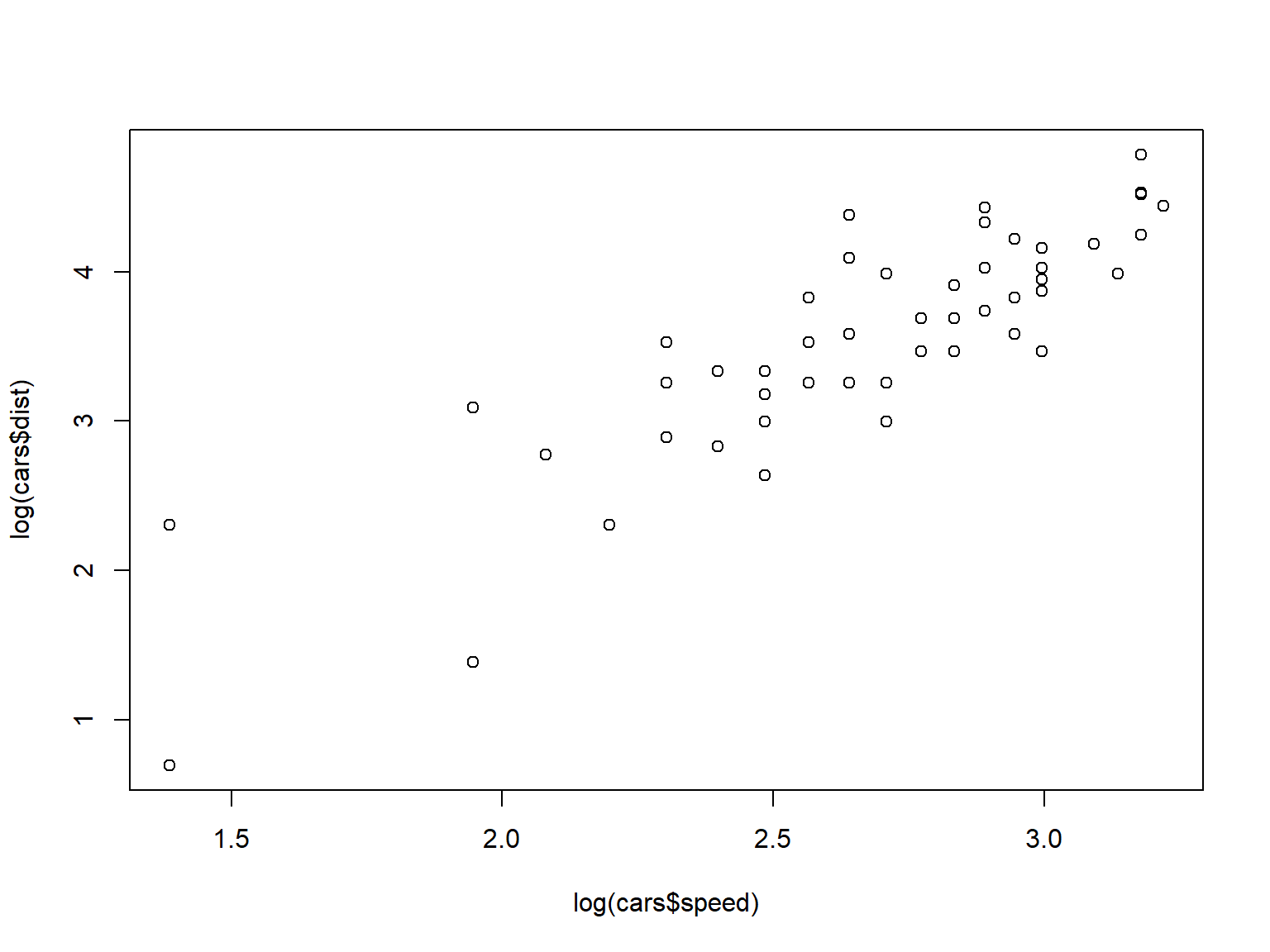
cor(log(cars$speed), log(cars$dist))
## [1] 0.8562385
dplyr - Introduction
dplyr is a commonly used package (which we need to load into R as it is not part of ‘base R’). It makes manipulating dataframes very easy and intuitive and is great for data analysis. To install (and load) any package, just type
# Install the package on your computer (not needed if you do this in Ed!)
install.packages('dplyr')
# Loads the package, you need this every time you use it
library('dplyr')
There are 6 main functions in dplyr:
filter - selects rows
select - selects columns
arrange - sorts rows by some order
mutate - creates new columns
group_by - groups certain rows together
summarise - provides summaries of grouped rows
dplyr - Filter and Select
Here some examples using the in-built data frame mtcars
# Show the dataset
head(mtcars)
##                    mpg cyl disp  hp drat    wt  qsec vs am gear carb
## Mazda RX4         21.0   6  160 110 3.90 2.620 16.46  0  1    4    4
## Mazda RX4 Wag     21.0   6  160 110 3.90 2.875 17.02  0  1    4    4
## Datsun 710        22.8   4  108  93 3.85 2.320 18.61  1  1    4    1
## Hornet 4 Drive    21.4   6  258 110 3.08 3.215 19.44  1  0    3    1
## Hornet Sportabout 18.7   8  360 175 3.15 3.440 17.02  0  0    3    2
## Valiant           18.1   6  225 105 2.76 3.460 20.22  1  0    3    1

# Filters the dataset for observations with mpg greater than 30
filter(mtcars, mpg > 30)
##                 mpg cyl disp  hp drat    wt  qsec vs am gear carb
## Fiat 128       32.4   4 78.7  66 4.08 2.200 19.47  1  1    4    1
## Honda Civic    30.4   4 75.7  52 4.93 1.615 18.52  1  1    4    2
## Toyota Corolla 33.9   4 71.1  65 4.22 1.835 19.90  1  1    4    1
## Lotus Europa   30.4   4 95.1 113 3.77 1.513 16.90  1  1    5    2

# Returns the dataframe mtcars but only with the 3 specified columns
select(mtcars, mpg, cyl, wt)
##                      mpg cyl    wt
## Mazda RX4           21.0   6 2.620
## Mazda RX4 Wag       21.0   6 2.875
## Datsun 710          22.8   4 2.320
## Hornet 4 Drive      21.4   6 3.215
## Hornet Sportabout   18.7   8 3.440
## Valiant             18.1   6 3.460
## Duster 360          14.3   8 3.570
## Merc 240D           24.4   4 3.190
## Merc 230            22.8   4 3.150
## Merc 280            19.2   6 3.440
## Merc 280C           17.8   6 3.440
## Merc 450SE          16.4   8 4.070
## Merc 450SL          17.3   8 3.730
## Merc 450SLC         15.2   8 3.780
## Cadillac Fleetwood  10.4   8 5.250
## Lincoln Continental 10.4   8 5.424
## Chrysler Imperial   14.7   8 5.345
## Fiat 128            32.4   4 2.200
## Honda Civic         30.4   4 1.615
## Toyota Corolla      33.9   4 1.835
## Toyota Corona       21.5   4 2.465
## Dodge Challenger    15.5   8 3.520
## AMC Javelin         15.2   8 3.435
## Camaro Z28          13.3   8 3.840
## Pontiac Firebird    19.2   8 3.845
## Fiat X1-9           27.3   4 1.935
## Porsche 914-2       26.0   4 2.140
## Lotus Europa        30.4   4 1.513
## Ford Pantera L      15.8   8 3.170
## Ferrari Dino        19.7   6 2.770
## Maserati Bora       15.0   8 3.570
## Volvo 142E          21.4   4 2.780

# Returns the columns mpg and cyl for rows with wt greater than 2
select(filter(mtcars, wt > 3, cyl >= 6), mpg, cyl, wt)
##                      mpg cyl    wt
## Hornet 4 Drive      21.4   6 3.215
## Hornet Sportabout   18.7   8 3.440
## Valiant             18.1   6 3.460
## Duster 360          14.3   8 3.570
## Merc 280            19.2   6 3.440
## Merc 280C           17.8   6 3.440
## Merc 450SE          16.4   8 4.070
## Merc 450SL          17.3   8 3.730
## Merc 450SLC         15.2   8 3.780
## Cadillac Fleetwood  10.4   8 5.250
## Lincoln Continental 10.4   8 5.424
## Chrysler Imperial   14.7   8 5.345
## Dodge Challenger    15.5   8 3.520
## AMC Javelin         15.2   8 3.435
## Camaro Z28          13.3   8 3.840
## Pontiac Firebird    19.2   8 3.845
## Ford Pantera L      15.8   8 3.170
## Maserati Bora       15.0   8 3.570
dplyr - Pipeline operator and Arrange
As you apply more operations to your dataframe, the nested functions you use can get hard to read.
Luckily, dplyr includes the useful pipeline operator %>% (orally referred to as “pipe”, such as in “A pipe B”). Think of it as “and then”.
# Take the dataframe, AND THEN filter for mpg greater than 30
mtcars %>% filter(mpg>30)
##                 mpg cyl disp  hp drat    wt  qsec vs am gear carb
## Fiat 128       32.4   4 78.7  66 4.08 2.200 19.47  1  1    4    1
## Honda Civic    30.4   4 75.7  52 4.93 1.615 18.52  1  1    4    2
## Toyota Corolla 33.9   4 71.1  65 4.22 1.835 19.90  1  1    4    1
## Lotus Europa   30.4   4 95.1 113 3.77 1.513 16.90  1  1    5    2

# Do the same, AND THEN select certain columns
mtcars %>%
  filter(mpg > 30) %>%
  select(mpg, wt)
##                 mpg    wt
## Fiat 128       32.4 2.200
## Honda Civic    30.4 1.615
## Toyota Corolla 33.9 1.835
## Lotus Europa   30.4 1.513

########################### arrange ##################################
# Sort the rows in ascending order of wt
mtcars %>%
  filter(mpg > 30) %>%
  arrange(wt)
##                 mpg cyl disp  hp drat    wt  qsec vs am gear carb
## Lotus Europa   30.4   4 95.1 113 3.77 1.513 16.90  1  1    5    2
## Honda Civic    30.4   4 75.7  52 4.93 1.615 18.52  1  1    4    2
## Toyota Corolla 33.9   4 71.1  65 4.22 1.835 19.90  1  1    4    1
## Fiat 128       32.4   4 78.7  66 4.08 2.200 19.47  1  1    4    1

# Sort the rows in descending order of wt
mtcars %>%
  filter(mpg > 30) %>%
  arrange(desc(wt))
##                 mpg cyl disp  hp drat    wt  qsec vs am gear carb
## Fiat 128       32.4   4 78.7  66 4.08 2.200 19.47  1  1    4    1
## Toyota Corolla 33.9   4 71.1  65 4.22 1.835 19.90  1  1    4    1
## Honda Civic    30.4   4 75.7  52 4.93 1.615 18.52  1  1    4    2
## Lotus Europa   30.4   4 95.1 113 3.77 1.513 16.90  1  1    5    2
dplyr - Mutate
mutate() allows you to easily create new variables (as function of other variables)
mtcars %>%
  mutate(double_wt = wt*2, # Creates a new variable called double_wt
         kms_per_gallon = mpg*1.61, # Creates a new variable called kms_per_gallon
         name = row.names(mtcars)) %>%  # Creates a new variable with names of the cars
  select(name, double_wt, kms_per_gallon)
##                                    name double_wt kms_per_gallon
## Mazda RX4                     Mazda RX4     5.240         33.810
## Mazda RX4 Wag             Mazda RX4 Wag     5.750         33.810
## Datsun 710                   Datsun 710     4.640         36.708
## Hornet 4 Drive           Hornet 4 Drive     6.430         34.454
## Hornet Sportabout     Hornet Sportabout     6.880         30.107
## Valiant                         Valiant     6.920         29.141
## Duster 360                   Duster 360     7.140         23.023
## Merc 240D                     Merc 240D     6.380         39.284
## Merc 230                       Merc 230     6.300         36.708
## Merc 280                       Merc 280     6.880         30.912
## Merc 280C                     Merc 280C     6.880         28.658
## Merc 450SE                   Merc 450SE     8.140         26.404
## Merc 450SL                   Merc 450SL     7.460         27.853
## Merc 450SLC                 Merc 450SLC     7.560         24.472
## Cadillac Fleetwood   Cadillac Fleetwood    10.500         16.744
## Lincoln Continental Lincoln Continental    10.848         16.744
## Chrysler Imperial     Chrysler Imperial    10.690         23.667
## Fiat 128                       Fiat 128     4.400         52.164
## Honda Civic                 Honda Civic     3.230         48.944
## Toyota Corolla           Toyota Corolla     3.670         54.579
## Toyota Corona             Toyota Corona     4.930         34.615
## Dodge Challenger       Dodge Challenger     7.040         24.955
## AMC Javelin                 AMC Javelin     6.870         24.472
## Camaro Z28                   Camaro Z28     7.680         21.413
## Pontiac Firebird       Pontiac Firebird     7.690         30.912
## Fiat X1-9                     Fiat X1-9     3.870         43.953
## Porsche 914-2             Porsche 914-2     4.280         41.860
## Lotus Europa               Lotus Europa     3.026         48.944
## Ford Pantera L           Ford Pantera L     6.340         25.438
## Ferrari Dino               Ferrari Dino     5.540         31.717
## Maserati Bora             Maserati Bora     7.140         24.150
## Volvo 142E                   Volvo 142E     5.560         34.454
dplyr - Why use the pipeline operator?
The pipeline operator makes it much easier to read what is going on. Note that the following two pieces of code achieve the same thing.
# No pipeline
arrange(select(filter(mtcars, mpg > 30), mpg, wt, cyl), desc(wt))
##                 mpg    wt cyl
## Fiat 128       32.4 2.200   4
## Toyota Corolla 33.9 1.835   4
## Honda Civic    30.4 1.615   4
## Lotus Europa   30.4 1.513   4
# With pipeline
mtcars %>%
  filter(mpg > 30) %>%
  select(mpg, wt, cyl) %>%
  arrange(desc(wt))
##                 mpg    wt cyl
## Fiat 128       32.4 2.200   4
## Toyota Corolla 33.9 1.835   4
## Honda Civic    30.4 1.615   4
## Lotus Europa   30.4 1.513   4
It is hard to quickly get what the first code is doing. In contrast, you can easily interpret the second code as:
take the mtcars dataset, and then
filter for mpg > 30, and then
select the columns mpg, wt, cyl, and then
arrange them by descending weight
dplyr - summarise and group_by
summarise() will give you summary statistics
mtcars %>%
  summarise(mean_mpg = mean(mpg),
            num_cars = n(),
            sd_wt = sd(wt))
##   mean_mpg num_cars     sd_wt
## 1 20.09062       32 0.9784574
group_by() is a very powerful function that will group rows into different categories. You can then use summarise() to find summary statistics of each group
mtcars %>%
  group_by(cyl) %>% # Group cars by how many cylinders they have
  summarise(avg_mpg = mean(mpg)) # Find the average mpg for each group (cyl)
## # A tibble: 3 x 2
##     cyl avg_mpg
##   <dbl>   <dbl>
## 1     4    26.7
## 2     6    19.7
## 3     8    15.1
Common summary statistics include:
mean() the averagesd() the standard deviationn() the count
dplyr Exercise 1
Using the in-built dataset quakes:
Find all the rows with magnitude (mag) greater or equal to 5.5
Display only the columns depth, mag and stations
dplyr Exercise 1 Solution
quakes %>% filter(mag>5.5) %>% select(depth,mag,stations)
##    depth mag stations
## 1    139 6.1       94
## 2     50 6.0       83
## 3     42 5.7       76
## 4     56 5.7      106
## 5    127 6.4      122
## 6    205 5.6       98
## 7    216 5.7       90
## 8    577 5.7      104
## 9    562 5.6       80
## 10    48 5.7      123
## 11   535 5.7      112
## 12    64 5.9      118
## 13    75 5.6       79
## 14   546 5.7       99
## 15   417 5.6      129
## 16   153 5.6       87
## 17    93 5.6       94
## 18   183 5.6      109
## 19   627 5.9      119
## 20    40 5.7       78
## 21   242 6.0      132
## 22   589 5.6      115
## 23   107 5.6      121
## 24   165 6.0      119
dplyr Exercise 2
Using the in-built data set mtcars:
Create a new variable which is the product of mpg times wt.
Find the mean and median of this new variable, but within each possible value of cyl. Do you notice something?
dplyr Exercise 2 solutions
mtcars %>%
  mutate(mpg_times_wt = (mpg*wt)) %>%
  group_by(cyl) %>%
  summarise(mean = mean(mpg_times_wt), med = median(mpg_times_wt))
## # A tibble: 3 x 3
##     cyl  mean   med
##   <dbl> <dbl> <dbl>
## 1     4  59.3  55.6
## 2     6  61.2  61.2
## 3     8  59.2  55.5
dplyr - Why use dplyr?
dplyr is generally easier to read and write than base R. The following codes do the same thing
dplyr:
new_df <- mtcars %>%
  mutate(name = rownames(mtcars),
         kmpl = mpg * 0.264172 * 1.60934) %>%
  filter(mpg > 30,
         wt < 2) %>%
  select(name,
         kmpl,
         disp,
         wt)
Base R:
new_df <- mtcars[mtcars$mpg > 30 & mtcars$wt < 2,]
new_df["kmpl"] <- new_df$mpg * 0.264172 * 1.60934
new_df <- new_df[, c("kmpl", "disp", "wt")]
In particular, group_by and summarise are easy to write with dplyr. They are significantly harder to write in base R:
dplyr:
new_df <- mtcars %>%
  group_by(cyl, gear) %>%
  summarise(avg_weight = mean(wt),
            sd_weight = sd(wt))
## `summarise()` has grouped output by 'cyl'. You can override using the `.groups` argument.
Base R:
avg_weight <- aggregate(mtcars$wt,
          by = list(cylinders = mtcars$cyl,
                    gears = mtcars$gear),
          FUN = mean)

names(avg_weight)[3] <- "Average_weight"

sd_weight <- aggregate(mtcars$wt,
           by = list(cylinders = mtcars$cyl,
                     gears = mtcars$gear),
           FUN = sd)

names(sd_weight)[3] <- "std_dev_weight"

new_df <- merge(avg_weight, sd_weight, by = c("cylinders", "gears"))
Or to count the number of observations within given intervals:
dplyr:
sample_data %>%
  mutate(ints = cut(height, breaks= c(140,150, 160, 170, 180, 190), right = F)) %>%
  group_by(ints) %>%
  summarise(n = n())
## # A tibble: 5 x 2
##   ints          n
##   <fct>     <int>
## 1 [140,150)     3
## 2 [150,160)    70
## 3 [160,170)    89
## 4 [170,180)    52
## 5 [180,190)    12
Base R:
res <- hist(height, plot=FALSE, breaks = c(140,150,160,170,180,190), right = F) # put the data in 5 categories
x   <- as.table(res$counts) # create the table
nn  <- as.character(res$breaks)
dimnames(x) <- list(paste(nn[-length(nn)], nn[-1],sep="-")) # add names to categories: this step is not straightforward!
x
## 140-150 150-160 160-170 170-180 180-190
##       3      70      89      52      12
Homework Exercise 1
Given a matrix A:
\[ A = \begin{bmatrix} 1 & 2 & 3 \\ 4 & 5 & 6 \\ 7 & 8 & 9 \\ 10 & 11 & 12 \end{bmatrix} \] What are the outputs of the following instructions:
Homework Exercise 2
Using the iris dataset:
- Find all the rows with
Sepal.Width greater than \(2.7\) and then sort by Sepal.Length
- For all the
setosa flowers, find the ratio between Sepal.Length and Sepal.Width, call this new variable ratio and display only columns ratio and Species
- Find the average
ratio between Sepal.Length and Sepal.Width for each species of flower
Homework Exercise 3
Import the dataset sample_data.csv:
- create a new column called
BMI, which is calculated by \[ \frac{Weight}{Height(m)^2} \]
- calculate the average
BMI for each of the 6 categories of cooked_fruit_veg for FEMALE individuals only
Homework Exercise 4
The built-in dataset ChickWeight records the weights of chicks (in the variable weight), as well as the type of diet (\(1, 2, 3\) or \(4\) in the variable Diet).
Provide summary statistics for the weight in diet groups \(1\) to \(4\). Can you say for sure that a given group of chicks is the heaviest?
Home work Exercise 5
In Ed, the dataset motor.df is already loaded in the script on your right. This dataset contains some information about a large number of vehicle insurance claims, by policy. Perform the following tasks:
Display the first 10 rows of the dataset motor.df, and have a look at the variables names.
Use the package dplyr to create a summary table (or “tibble”) which should have two columns:
- The first reports the occurrence date of the accident, or
AccidentDay, but converted to the ‘date’ format. Hint: use function as.Date().
- The second is named
nc and reports, by AccidentDay, the total number of claims on each day.
- Use the table created in Q2 as well as function
plot() to produce a scatterplot of the daily numbers of CTP claims (y axis) from the year 2006 to the year 2015 (x axis is time).
Additional Notes: The which() function for matrices - Page 104
m <- matrix(c(1,2,3,1,2,3,2,1,3),3,3)
m
##      [,1] [,2] [,3]
## [1,]    1    1    2
## [2,]    2    2    1
## [3,]    3    3    3
which(m == 1)
## [1] 1 4 8
# m is seen as the concatenation of its columns
which(m == 1,arr.ind=TRUE)
##      row col
## [1,]   1   1
## [2,]   1   2
## [3,]   2   3
# this gives the indices (row and column) of all elements = 1